To analyze time series data, it is always useful to identify what kind of process are we seeing: White noise, moving average, autoregressive, or a combination of the last two, autoregressive moving average. If we simply try to visualize these processes, it will be almost impossible to distinguish them from one another.

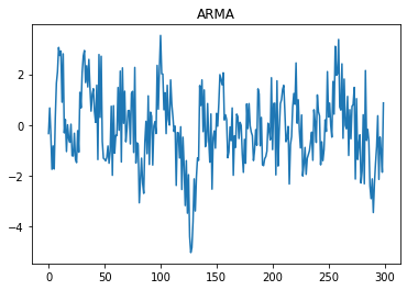
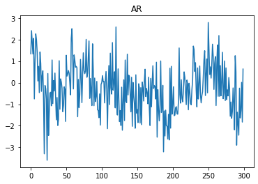
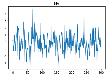
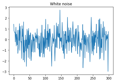
For example, the images above were generated using the following formulas:

• Autoregressive moving average: \[ y_{t} = 0.1y_{t-1} + 0.2y_{t-2} + 0.3y_{t-3} + \epsilon_{t} + 0.1\epsilon_{t-1} + 0.2\epsilon_{t-2} + 0.5\epsilon_{t-3} + 0.05\epsilon_{t-4} \]
• Autoregressive:
  \[ y_{t} = 0.1y_{t-1} + 0.2y_{t-2} + 0.3y_{t-3} + \epsilon_{t} \]
• Moving average:
  \[ y_{t} = \epsilon_{t} + 0.1\epsilon_{t-1} + 0.2\epsilon_{t-2} + 0.5\epsilon_{t-3} + 0.05\epsilon_{t-4} \]
• White noise:
  \[ y_{t} = \epsilon_{t} \]

Even though the formulas that generated these 4 processes are different, it is hard to categorize each process correctly by sight. To begin disentangling the inner structures of each series, we need to resort to autocorrelation functions, but to understand them, we first need to understand autocovariance functions.

Autocovariance function

The word autocovariance seems complicated but is just a sophisticated way of naming the calculation of the covariance of a series with itself (but lagged $j$ periods). We can define the autocovariance function ($\gamma_{j}$) as:

\[ \gamma_{j} = Cov(y_{t}, y_{t-j}) = E[(y_{t} - \mu_{t})(y_{t-j} - \mu_{t-j})] \]

Here, $y_{t}$ is the original series, $y_{t-j}$ is the same series lagged $j$ periods, and $\mu_{t}$ and $\mu_{t-j}$ are their corresponding means.
If we assume that the series is weakly stationary¹, we can now simplify the expression to:

\[ \gamma_{j} = E[(y_{t} - \mu)(y_{t-j} - \mu)] \]

To estimate $\gamma_{j}$, we use the sample autocovariance function:

\[ \hat{\gamma_{j}} = \frac{1}{n}\sum_{t=j}^{n} (y_{t} - \bar{y})(y_{t-j} - \bar{y}) \]

Here, $\bar{y}$ is the sample mean of the observations, and $n$ is the number of observations.

Autocorrelation function

Autocorrelation functions are just a normalization of autocovariance functions, this makes them have no unit of measurement (dimensionless). They are no more than the time series version of the typical Pearson correlation coefficient. Mathematically, we can define them as:

\[ \rho_{j} = \frac{\gamma_{j}}{\gamma_{0}} \]

The sample version of this is simply:

\[ \hat{\rho_{j}} = \frac{\hat{\gamma_{j}}}{\hat{\gamma_{0}}} \]

It is clear—but worth remembering—that always $\rho_{0} = \hat{\rho_{0}} = 1$.

Coding the calculation

I created two simple Python functions to do the calculations².

Autocovariance function

import numpy as np  # For clearness, imports will only be shown in this snippet.

def autocovariance(series, lag):
    len_series = len(series)
    mean_series = np.mean(series)

    covariances = []
    for index in range(lag, len_series):
        # Simple covariance calculation. This can be easily replaced with np.cov,
        # but it is educational to calculate it ourselves.
        covariance = (series[index] - mean_series) * (series[index - lag] - mean_series)
        covariances.append(covariance)

    autocovariance = np.sum(covariances) / len_series
    return autocovariance

Autocorrelation function

def autocorrelation_function(series, max_lags=20):
    lag_list = list(range(max_lags))
    autocovariances = []
    for lag in lag_list:  # Calculating autocovariances for each lag
        autocovariances.append(autocovariance(series, lag))

    autocorrelations = np.divide(autocovariances, autocovariances[0])
    return autocorrelations

Visualizing and analyzing the functions

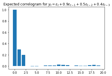
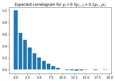
Finally, we can visualize the autocorrelation function of each of the series shown in the beginning³:

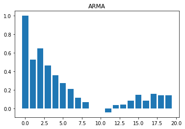
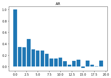
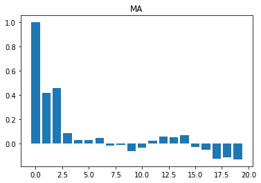
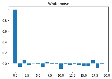
Now it is clear that the four series are different. Here are some simple rules to identify the times series structure by observing the autocorrelation function composition:

• White noise:
  We expect to see near-zero values for all $j>1$.
• Moving average:
  We should see near-zero values for all $j>q$, where $q$ is the number of lags. For example, if we have $y_{t} = \epsilon_{t} + 0.9\epsilon_{t-1} + 0.5\epsilon_{t-2} + 0.4\epsilon_{t-3}$, only the first three bars should be far from zero.

• Autoregressive:
  We should see an exponential decay to zero; there are no other explicit guidelines. This is the reason autocorrelation functions are not extremely useful to discover the structure of autoregressive processes. (For a better understanding of these kinds of processes, we need to resort to partial autocorrelation functions.)
  As an example, if we have $y_{t} = 0.5y_{t-1} + 0.2y_{t-2} \epsilon_{t}$, we will see the bars slowly reaching near-zero values.

• Autoregressive moving average:
  We expect a slow decay. Normally, it is hard to disentangle the effect of the different parameters.

Autocorrelation functions are a good first approximation to analyze time series data, but they are just that: “a first approximation.” There are other methods to continue finding the right structure of our data, for example, the Akaike Information Criterion or the Bayesian Information Criterion.

You can find all the code here and play with an online Jupyter Notebook here .