Dickey-fuller table using Monte Carlo

One critical aspect of time series analysis is to determine if we are dealing with a unit root or not. If we fail to consider this, we may end up with all of our tests and conclusions invalidated!¹
To begin understanding how to test our data for a unit root, let us consider the following $AR(1)$ process as our base scenario: \[ y_t = \alpha + \rho y_{t-1} + \epsilon_t \]

In this model, checking for a unit root is translated into testing $\rho = 1$ . We can define our hypothesis as:

\[ H_0: \rho = 1\\
H_1: |\rho| < 1 \]

Seeing this simple problem, we can be tempted to run OLS on the base model and see if $\rho = 1$ using a t-test. The problem with this approach is that under the null hypothesis, $y_t$ and $y_{t-1}$ are non-stationary, so we cannot simply apply the central limit theorem, and thus our t-test is invalid.
We can modify our base model to our advantage by subtracting $y_{t-1}$ on both sides of the equation:

\[ \begin{align} y_t - y_{t-1} &= \alpha + \rho y_{t-1} - y_{t-1} + \epsilon_t\\
\Delta y_t &= \alpha + (\rho - 1) y_{t-1} + \epsilon_t \end{align} \]

Notice that in the last equation, under the null hypothesis (i.e. $\rho = 1$ ) the variable $y_{t-1}$ disappears and makes $\Delta y_t$ stationary. Keep in mind that $y_t$ and $y_{t-1}$ are still non-stationary, it is just that the difference between $y_t$ and $y_{t-1}$ is stationary. To make this more clear, observe that under the null hypothesis $\Delta y_t = \alpha + \epsilon_t$ . The right-hand side of the equation is stationary!
Additionally, under the alternative hypothesis (i.e. $|\rho| < 1$ ) the variable $y_{t-1}$ does not disappear, but this is no longer a problem because $y_{t-1}$ is stationary (by definition of the alternative hypothesis).

We still cannot use a t-test on our last equation to verify if $(\rho - 1) = 0$ , but we are getting closer. For convenience, we define $\delta = \rho - 1$ :

\[ \Delta y_t = \alpha + \delta y_{t-1} + \epsilon_t \]

The problem with this is that under the null hypothesis $y_{t-1}$ is still non-stationary, and thus $\hat{\delta}$ does not have a t-distribution. Thanks to David Dickey and Wayne Fuller, we now know that it has a defined distribution (i.e. the Dickey-Fuller distribution). This means that we can simply calculate a t-statistic and compare it to the critical values of a Dickey-Fuller table.

The Dickey-Fuller test is one of the simplest tests to determine if a time series has a unit root or not. The only difference with the reasoning presented above is that the test involves 3 alternative hypotheses²:

An autoregressive process with parameter $\rho < 1$ , mean equal to zero and no trend: \[ \Delta y_t = (\rho - 1) y_{t-1} + \epsilon_t \]
An autoregressive process with parameter $\rho < 1$ , non-zero mean and no trend: \[ \Delta y_t = \alpha + (\rho - 1) y_{t-1} + \epsilon_t \]
An autoregressive process with parameter $\rho < 1$ , non-zero mean and trend: \[ \Delta y_t = \alpha + \beta t + (\rho - 1) y_{t-1} + \epsilon_t \]

Monte Carlo method to get a Dickey-Fuller table

Description of the method

In simple words, to get our Dickey-Fuller distributions and our critical values, we need to simulate many $AR(1)$ processes with a unit root (i.e. with $\rho = 1$ ) and then we need to try to assess how likely it is to observe $\rho = 0$ due to the randomness of the simulation.

Here is a step-by-step outline of the process³:

Simulate an $AR(1)$ process of length $N$ with $\rho = 1$ .
Calculate $\Delta y_t = y_t - y_{t-1}$ .
Run one regression for each model:
- $\Delta y_t = \delta y_{t-1} + \epsilon$ → save the t-statistic of $\hat{\delta}$ .
- $\Delta y_t = \alpha + \delta y_{t-1} + \epsilon$ → save the t-statistic of $\hat{\delta}$ .
- $\Delta y_t = \alpha + \beta t + \delta y_{t-1} + \epsilon$ → save the t-statistic of $\hat{\delta}$ .
Repeat steps 1-3 as many times as necessary (probably at least 10,000 or 20,000 times).
To calculate the critical value of a model (for a defined $N$ ) at $\alpha\%$ , calculate the $\alpha$ percentile of each group of t-values.

Implementing the code

Here is a small Python program that accomplishes the steps listed above⁴.

import statsmodels.api as sm
import numpy as np
import pandas as pd
import matplotlib.pyplot as plt

from ARMA import ARMA  # Custom module to simulate series. Can be replaced with statsmodels.
                       # See repository for more details.
repetitions = 10000
models = ['model_a', 'model_b', 'model_c']
series_lengths = [25, 50, 100, 250, 500]
percentiles = [10, 5, 2.5, 1]

# Creating an empty list for each model and length.
# t_values = {'model_a': {25: [], ...}, 'model_b': {25: [], ...}, ...}
t_values = {model: {series_length: [] for series_length in series_lengths} for model in models}

for series_length in series_lengths:
    for __ in range(repetitions):

        y = ARMA.generate_ar(series_length, [1])  # y_{t} = y_{t-1} + e_{t}
        delta_y = np.diff(y)  # delta_y_{t} = y_{t+1} - y_{t}
        alpha = np.ones(series_length)  # alpha = 1
        beta_t = np.arange(series_length)  # beta*t = [0, 1, 2, ...]

        # Model a:
        regressors_a = y[:-1]  # This makes y and delta_y have the same size.
        results_a = sm.OLS(delta_y, regressors_a).fit()
        t_values['model_a'][series_length].append(results_a.tvalues[0])

        # Model b:
        regressors_b = np.column_stack((y, alpha))[:-1]
        results_b = sm.OLS(delta_y, regressors_b).fit()
        t_values['model_b'][series_length].append(results_b.tvalues[0])

        # Model c:
        regressors_c = np.column_stack((y, alpha, beta_t))[:-1]
        results_c = sm.OLS(delta_y, regressors_c).fit()
        t_values['model_c'][series_length].append(results_c.tvalues[0])

# Creating an empty DataFrame to store the critical values.
index = pd.MultiIndex.from_product([models, series_lengths])
df_table = pd.DataFrame(columns=percentiles, index=index)

# Filling the DataFrame.
for model in models:
    for series_length in series_lengths:
        for percentile in percentiles:
            critical_t_value = np.percentile(t_values[model][series_length], percentile)
            df_table.loc[(model, series_length), percentile] = critical_t_value

To get our table, we can simply do:

df_table.astype(float).round(2)

Model	N	10%	5%	2.5%	1%
Model a	25	-1.61	-1.96	-2.28	-2.66
	50	-1.61	-1.95	-2.24	-2.61
	100	-1.62	-1.95	-2.24	-2.59
	250	-1.62	-1.95	-2.24	-2.58
	500	-1.62	-1.94	-2.23	-2.57
Model b	25	-2.64	-2.99	-3.32	-3.73
	50	-2.60	-2.92	-3.22	-3.57
	100	-2.58	-2.89	-3.16	-3.49
	250	-2.57	-2.87	-3.13	-3.45
	500	-2.57	-2.87	-3.13	-3.44
Model c	25	-3.24	-3.61	-3.95	-4.39
	50	-3.18	-3.50	-3.80	-4.15
	100	-3.15	-3.46	-3.73	-4.06
	250	-3.14	-3.43	-3.69	-4.00
	500	-3.13	-3.42	-3.67	-3.98

To plot each distribution, we can use matplotlib:

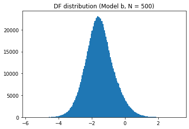
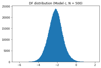
sel_length = 500

for model_name in models:
    plt.hist(t_values[model_name][sel_length], bins=200)
    plt.show()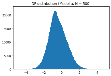

You can find all the code here and play with an online Jupyter Notebook here .
You can also find a Matlab version of the code here .

The presence of unit roots makes our time series non-stationary, which in turn makes inference much harder and less straightforward. ↩
The reason behind this is that the Dickey-Fuller distribution depends on the type of model (a, b or c) and the length of the series. ↩
I got the idea of the description from here (the description is for a similar test). ↩
On my laptop, 100,000 repetitions took about 15-20 minutes. ↩