An important part of Econometrics focuses on analyzing time series. We can apply time series analysis to almost any context, the only requirement is that we have similar data along different periods.
To analyze and understand time series, it is sometimes useful to simulate data. In its simplest form, we can classify them into 4 categories: white noise, autoregressive, moving average, and a combination of the last two, called—unsurprisingly—autoregressive moving average.
Even though many programs that can already perform these simulations out-of-the-box (STATA, Matlab, Python modules, etc.), it is still interesting to develop them on our own. With this aim in mind, I developed a simple Python class that can simulate the series described.

White noise process

A white noise process is as simple as it can get: it is just random numbers (which are sometimes called “innovations”). As a curious side note, the term “white noise” is not original from time series. It was first used to describe a sound that had all frequencies together¹.
For our context, we will define a “white noise” as:

yt=ϵt

Where ϵt satisfies the following properties:

E[ϵt]=E[ϵt|ϵt−1,ϵt−2,…]=0V[ϵt]=V[ϵt|ϵt−1,ϵt−2,…]=σ2E[ϵtϵt−j]=E[ϵtϵt−j|ϵt−1,ϵt−2,…]=0with j≠0

Equation (1) guarantees that the process has a conditional mean of zero. Equation (2) that the process has a constant variance (homoscedastic), and equation (3) that errors are uncorrelated. It is worth noticing that no distribution is imposed on ϵt, but to keep things simple, we will use a normal distribution with a variance of 1. Here is that definition written in code:

import numpy as np  # For clearness, imports will only be shown in this snippet.

def generate_wn(n, sigma=1):
    return np.random.normal(0, sigma, size=n)  # The first parameter makes E[e_t] = 0.

Moving average process

In simple words, a moving average process is just a weighted combination of values coming from a white noise process. Mathematically, we define a moving average process of q lags (also called MA(q)) as:

yt=μ+ϵt+θ1ϵt−1+θ2ϵt−2+…+θqϵt−q

Here, each θt tells us how much the series “remembers” each ϵt. We add the parameter μ to allow the process to have a non-zero mean.
To simulate a moving average process we need to:

1. Generate a white noise series.
2. Weight and sum the values of the white noise process.
3. Remove the first q elements of the series (q being the number of coefficients used).

Here are the steps listed above, now written in code:

def generate_ma(n, thetas, mu, sigma=1):
    q = len(thetas)
    adj_n = n + q  # We add q values because at the beginning we have no thetas available.
    e_series = ARMA.generate_wn(adj_n, sigma)  # Generating a white noise.

    ma = []
    for i in range(1, adj_n):
        visible_thetas = thetas[0:min(q, i)]  # At first, we only "see" some of the thetas.
        visible_e_series = e_series[i - min(q, i):i]  # The same happens to the white noise.

        reversed_thetas = visible_thetas[::-1]

        try:  # Getting e_t if we can.
            e_t = visible_e_series[-1]
        except IndexError:
            e_t = 0

        # Main equation.
        ma_t = mu + e_t + np.dot(reversed_thetas, visible_e_series)

        ma.append(ma_t)

    ma = ma[max(q-1, 0):]  # Dropping the first values that did not use all the thetas.

    return ma

Autoregressive process

An autoregressive process consists in starting with an arbitrary number and using past results to generate iteratively future values. The parameters of this function determine how much the series “remembers” itself. Mathematically, we define an autoregressive process of p lags (also called AR(p)) as:

yt=ϕ1yt−1+ϕ2yt−2+…+ϕpyt−p+ϵt

Here, each ϕt tells us how much the series weights its past values, and ϵt is a simple random number. To simulate a moving average process, we need:

1. Start with an arbitrary value for y0.
2. Generate a white noise process.
3. Determine each new yt using yt−1,yt−2,... and ϵt.
4. Remove the first p elements of the series (p being the number of coefficients used).

Here are the steps listed above, now written in code:

def generate_ar(n, phis, sigma=1):
    p = len(phis)
    adj_n = n + p  # We add q values because at the beginning we have no phis available.
    e_series = ARMA.generate_wn(adj_n, sigma)  # Generating a white noise.

    ar = [e_series[0]]  # We start the series with a random value
    for i in range(1, adj_n):
        visible_phis = phis[0:min(p, i)]  # At first, we only "see" some of the phis.
        visible_series = ar[i - min(p, i):i]  # The same happens to the white noise.

        reversed_phis = visible_phis[::-1]

        # Main equation.
        ar_t = e_series[i] + np.dot(reversed_phis, visible_series)

        ar.append(ar_t)

    ar = ar[p:]  # Dropping the first values that did not use all the phis.

    return ar

Autoregressive moving average process

As the name suggests, this process is just a combination of the last two. This means that it has “memory” over its past values and also over the innovations. Mathematically, we define an autoregressive moving average process of p lags in y, and q lags in ϵ (noted as ARMA(p,q)) as:

yt=μ+ϕ1yt−1+ϕ2yt−2+…+ϕpyt−p+ϵt+θ1ϵt−1+θ2ϵt−2+…+θqϵt−q

To simulate this process, we just need to sum each sub-process in each instance:

def generate_arma(n, phis, thetas, mu, sigma=1):
    p = len(phis)
    q = len(thetas)

    adj_n = n + max(p, q)  # We use max to make sure we cover the lack of coefficients.
    e_series = ARMA.generate_wn(adj_n)  # Base white noise.

    arma = [e_series[0]]  # We start the series with a random value (same as AR).
    for i in range(1, adj_n):
        visible_phis = phis[0:min(p, i)]
        visible_thetas = thetas[0:min(q, i)]

        reversed_phis = visible_phis[::-1]
        reversed_thetas = visible_thetas[::-1]

        visible_series = arma[i - min(p, i):i]
        visible_e_series = e_series[i - min(q, i):i]

        try:  # Getting e_t if we can.
            e_t = visible_e_series[-1]
        except IndexError:
            e_t = 0

        # Main equation.
        ar_t = + np.dot(reversed_phis, visible_series)
        ma_t = mu + e_t + np.dot(reversed_thetas, visible_e_series)
        arma_t = ar_t + ma_t

        arma.append(arma_t)

    arma = arma[max(p, q):]  # Dropping the first values that did not use all the phis or thetas.

    return arma

Plotting the series

Finally, we can visualize the series created:

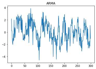
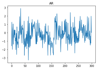
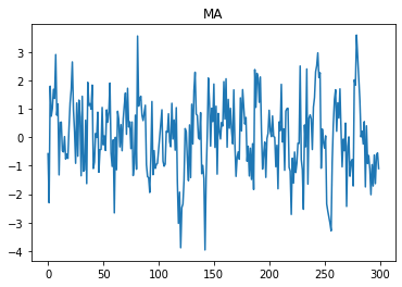
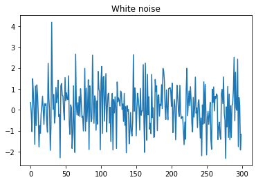
What is interesting is that it is difficult to distinguish each process just by looking at the plot. To visually differentiate the series, we can resort to a visual tool called correlograms.

You can find all the code here and play with an online Jupyter Notebook here .
You can also find a Matlab version of the code here .